
LECTURE 3 : Be Careful What You Wish For

Each of these lectures is designed to have a distinct theme rather than concentrating on a specific topic. In the first lecture we looked at what we know about galaxies and the processes that affect them with some high degree of confidence, and in the second we looked at how we know what it is that we think we know. Today's theme is why we interpret the data to mean what we think it means; it will be somewhat more philosophical than the other lectures (although don't expect anything very deep from this). This means I'll be jumping between topics a bit more than usual. Some of what I'll describe here is more relevant as an introduction to the final lecture. But I'll try not to go too overboard with this; everything will be grounded in an introduction to galaxy evolution theory - the ideas of monolithic collapse, hierarchical merging, the basics of how simulations work, and how conditions in the early Universe meant that processes affecting galaxies were different to the ones we see in operation today.
The reason I've decided to do it this way is because in extragalactic astronomy we can't do experiments. We can't fly to our subjects to examine them more closely or from another angle. We can't wait millions of years to see if our theoretical predictions come true. And we certainly can't do controlled experiments on our subjects. So all of our predictions can only be tested statistically. Understanding the statistical biases we may encounter, and how that influences our theory (and while biases affect observations as well, the most extreme case of all is how we compare theory and observation), is vital if we're to have any chance of working out what's really going on. If we don't account for this, then just like the scientists in Jurassic Park, we'll probably get eaten by a velociraptor. Or devoured by a hungry galaxy or something, I don't know.

Where did it all go wrong ?
At the end of one of the "history of astronomy" slides in the first lecture, I mentioned that after around the 1980's, everything started to go horribly wrong. Of course this isn't literally true : there have been many very important discoveries since then. But that was when numerical simulations really started to become important for extragalactic studies, and ever since then some major problems have emerged that are still with us today.
It seems appropriate to start with a (very) brief history of numerical simulations. The image below shows the very first extragalactic simulation. Before you scroll down (or click on the link), have a guess as to when it was performed. I'll give you a clue : it was earlier than the 1980's.
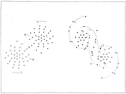
This result actually comes from 1941 and was performed using light bulbs. I love this. It's one of my favourite anecdotes : this crazy astronomer Erik Holmberg (okay, not literally crazy, but ridiculously dedicated) was so determined to run a numerical simulation that, dammit, he wasn't willing to wait for computers to be invented. Although they had crude mechanical computing devices at the time (not everything had to be done by hand), the calculations were just too demanding. Holmberg realised that he could greatly simplify one of the steps. He noticed that the intensity of light from a light bulb decays as 1/r2, exactly like the force of gravity. So by setting up this array of light bulbs, and using an electronic instrument to measure the intensity of light at each point, he could measure the total brightness and use that as a proxy for gravitational acceleration.
Of course, he still had a lot of work to do. He had to then go away and calculate how to move all these light bulbs assuming that the acceleration remained constant for some short, fixed interval. Then he had to reposition all the light bulbs by hand and do the whole damn thing again. Of course his result is impossibly crude by today's standards, with just 37 points per galaxy. But the workload... my God, this must have been absolutely immense. It was a truly heroic effort for what was really not all that an impressive result.
It wasn't no result at all, mind you. He found that two interacting discs could induce the formation of spiral arms, which is not so different from some modern theories of spiral arm formation. But with only 37 particles per galaxy, and a terrifying amount of effort required, no-one else attempted another simulation for 20 years.
It wasn't until the 1960's that the modern electronic programmable computer really started to come on to the scene. Those early simulations were not all that much better than Holmberg's : until the late 1970's, they were limited to a few hundred (perhaps a few thousand) particles with the physics limited to pure gravity. Computers were just not up to the job of including the much more complicated hydrodynamical forces needed to properly simulate the gas. Here's an early simulation using 700 particles to simulate the formation of a galaxy cluster :

Towards the end of the 70's, things started to improve - tens of thousands and even hundreds of thousands of particles became possible. After that, things advanced very quickly, bringing us in to the modern era. There's not really any point in going through a detailed history, so let's cut to what we can do today.
A really big modern simulation can have up to a trillion particles. That's at the extreme limit, of course, and many smaller simulations are still run on ordinary desktop machines. These smaller experiments are extremely useful, because you don't have to apply for time on one of these big supercomputers - you can just do whatever experiment you need and play around in a way that you can't do with time awarded on an expensive computing cluster. Desktop simulations routinely use a few hundred thousand or perhaps a few million particles.
As well as the increased particle number, modern simulations can also use far more complex physics. They still use n-bodies for the dark matter and stars, but the complex hydro-physics of the gas can also be simulated (I'll describe the basics of how this is done later). They can include heating and cooling, as well as chemical evolution due to the stars which changes the cooling and influences the star formation. They can even include magnetic fields.
 |
| From the Illustris simulation. |
Keep It Simple, Stupid
Starting out with these hugely complicated models would be a mistake. It's better to go with a well-established principle of science that works for a lot of other things too : KISS; Keep It Simple, Stupid. Start out with the simplest possible model and only add complexity later. That might not get you the right result straight away, but it will at the very least help understand how each process works independently before you tackle what happens when they're all going on at the same time.
So what the first big simulations of the evolution of the Universe did was to only use dark matter. Here's an example from the Millennium Simulation, which used 10 billion n-body particles. There's nothing here except gravity :
It begins in the early Universe with a more-or-less uniform density field, with some small variations caused by quantum fluctuations from soon after the Big Bang. Over time, it very naturally reproduces the observed structure of filaments and voids we see today.
This model is justified for two reasons. First, the dark matter is overall thought to be about 5x more massive than the baryons, so including them shouldn't make much difference to the overall result. In fact on the smaller scales of individual galaxies the dark matter can be much more dominant than that, at the level of a factor of 100-1,000. I was hoping to be able to talk about where the other baryons went in the final lecture but there wasn't time, but you can read a summary here.
Second, this model requires only very simple physics. Adding in the baryons on the scales shown here is just not computationally possible (or at least it wasn't at the time). And of course, it's also justified because it seems to work. The filaments and voids we observe in reality form naturally in the simulations with just gravity. There doesn't seem to be any need to add in anything more complicated.
Of course, as mentioned last time this model works well on large scales but is pretty lousy on smaller scales. If we zoom in to that same simulation :
At first it looks like we have a sort of fractal structure, with filaments being seen on ever smaller scales. But at some point a limit is reached and the filaments disappear, and on the scale of galaxy groups the distribution of the subhalos is approximately isotropic. And we know that that isn't what we see. As discussed last time, we don't see hundreds and hundreds of tiny galaxies around the Milky Way, we see about 50.
When people first started these kinds of simulations back in the early 1990's, there were problems getting any substructure to form at all. But that turned out to be an effect of resolution : they just didn't have enough particles, so they weren't able to resolve the very smallest structures. Once computational power increased a few years later, the problem ever since has been forming too much substructure - roughly a factor of 10 compared to observations.
The fundamental difficulty, of course, is that this model only contains dark matter, whereas what we detect observationally are stars and gas. So how do we go about relating this pure dark matter to what we see in reality ?
The missing satellite problem
The problem is that the two data sets are very different. Observationally we have many different complex parameters : stellar mass, luminosity, colour, 3D spatial position, line-of-sight velocities, morphology, gas mass, etc. But the simulations give us something much simpler : dark matter particle position, masses, and velocities, and that's just about all. We need to find a like-for-like comparison between these two data sets.
We also know that that baryonic mass is very much less than the dark matter mass, so we can't really compare masses directly. And the baryonic physics is very complicated, so we can't (for now) add it in to the simulations.
The most popular method for these early simulations was to use so-called semi-analytic models. An analytic model is, of course, just an equation - an analytic expression. The "semi-analytic" bit just refers to the fact that here these equations are used in conjunction with the numerical models. So for each dark matter halo, some recipe can be used to calculate the baryonic mass, which can then be compared with observations.
These models can be extremely simple but they can also be incredibly sophisticated. For example, the simplest possible case would be to give every halo some fixed baryonic mass fraction, so all you'd have to do is calculate its dark matter mass. A more sophisticated model might also account for the halo's environment, e.g. whether it was in a filament, void or cluster, and try and account for the environmental processes that might alter its baryonic content. You could even - at least in principle - try and account for the merger history of the object in some way, and whether the halo experiences an AGN or a strong feedback from star formation. What these models can't really do, however, is account for the baryons in other halos affecting them, and sometimes the geometry of a situation demands a true numerical model to solve accurately.
Once you do that, on the large-scale the filamentary structure doesn't look much different in visible light, which is good :
 |
| Dark matter on the left, predicted visible light on the right. |

So these semi-analytic models haven't helped, despite being surprisingly sophisticated. Darn ! Our other options are more drastic. We could concede that we have to include the baryonic physics, though that will mean waiting for more computational power. We could resort to concluding that because our model doesn't match reality, it must be completely wrong so we should chuck it out and try a completely different approach. And some people do that, which I'll look at later and in the next lecture. Another option, perhaps a bit milder, is to change our interpretation of the model : not quite all the subhalos host galaxies, so might this difference be stronger in reality ? Could we find some reason why this might be the case without having to throw out our idea completely ?
This is a hugely complicated problem, and we should start with some simpler cases first. We don't want to dive in to the complex baryonic physics we might need to include without first examining how the simulations themselves work first. We also need to understand the limitations of both simulations and observations before we tackle how to compare them to each other, as well as to decide when we need to throw away a theory and we can legitimately modify it.
Simulations aren't magical (they're just very complicated)
Especially as an observational astronomer, it's easy to be seduced by the power of simulations and think that theorists live in a wonderful realm free of the limits that plague observers. Their principle advantage is time evolution, something that observations just can't do.
Which is great, but simulations have all kinds of limitations, just as many as observations do. For starters, the intrinsic resolution effects mean that it's just not always possible to reproduce reality even if all the physics was perfectly understood (which it never is). We've already seen how substructure couldn't form in those early simulations which had poor mass resolution. These days, n-body simulations are still used (especially for things like star clusters which have little or no gas) but including baryonic physics is now pretty normal - at least on small scales if not in cosmological volumes. And they generally don't include all of the baryonic physics we know about - simplifications have to be made by necessity, though with the hope that things are not being made to be too simple.
Resolution effects can be more subtle for gas than in the case of n-bodies. In reality, gas is composed of a finite but immense number of discrete particles. In (some) simulations, the gas is composed of particles but using a vastly lower number than in reality. This means that its internal friction does not accurately model what would actually occur, so an artificial viscosity has to be introduced to try and reproduce it.
Another resolution limit is the need to use star particles, which are not the same as stars. We can't simulate the formation of individual star on galaxy-scale simulations - there would just be too many (400 billion or so in the Milky Way) and we don't have the resolution. So a star particle is more like a star cluster. This changes how they gravitationally interact with one another and how they accumulate mass from the interstellar medium and inject energy and matter back in to it. In reality star clusters are significantly extended, so their interactions in the simulations are different to those in reality.
Increasing the number of particles is always possible in principle but not necessarily in practise. Computational time and power is limited, so you always reach some hard limit beyond which you just have to accept that your simulations are flawed.
Even though you know all the physics you put in, interpreting the result of a simulation is not always straightforward. But I'll discuss that more in a minute.
The important point is that, once you accept that your simulations may not be capable of reproducing reality in at least some aspects, you have to try and find a way to make a sensible, like-for-like comparison between simulations and observations. Here's a comparison between the simulation above and the galaxy known as Auriga's Wheel :

In this case nothing sophisticated was done - I just chose the colours in the simulation to try and resemble the observations. The structural comparison is fair (the position of the galaxy and the shape of the ring) but the colours are fictitious. If you want a proper, quantitative comparison, you need to make what are called synthetic observations. That is, you try and account for all the viewing effects and reconstruct what you would see using a real telescope.
This adds another level of complexity. First, you need to understand even more physics of your simulation. For example gas in simulations is generally treated as a single, uniform generic "gas" component - in reality you might be interested in something much more specific, like the carbon content of the gas or whether it's molecular or atomic, but these details can't usually be simulated directly. Or if you want a proper, quantitative estimate of the optical colours, you need to understand the luminosity functions of the stars so that you can work out how many stars of different brightnesses (and so colours) would be present in each star particle. This extra physics potentially adds more uncertainties.
Second, you also need a good knowledge of the observations you're trying to simulate, which is also non-trivial. We saw last time how the differences between interferometers and single dish observations greatly affect the results, and how drift scanning versus pointed observations leads to very different noise characteristics. I'll look at how complicated quantifying sensitivity can be later on, but the point is that this too adds more uncertainty.
All this makes it worthwhile to understand simulations in a bit more detail.
Practical methods of simulations
Although baryonic physics is now generally standard, n-body simulations still have many uses. They are not as simple as you might naively imagine. The goal is to increase n as much as possible whilst keeping computational time to a minimum, which is not so easy. For example, imagine a binary system orbiting a third object at a much larger distance. The binary system requires a very small timestep to accurately model its behaviour, whereas its motion around the third object doesn't require such precision. Optimising systems like this is not trivial.
Including the gas physics is even more complex. There are two basic techniques :
Smoothed Particle Hydrodynamics
In reality the gas is composed of a finite yet immense number of particles. The SPH approach is to approximate the gas by some much smaller particle number. To better model the hydrodynamic fluid effects in real gas, each particle is deemed to be part of a kernel of other particles, usually containing some fixed number of particles (say, 50). The hydrodynamic equations - which I won't go in to - for the variation in density, temperature, pressure and so velocity, are then solved for the different kernels. In this way the discrete set of particles is effectively transformed into something closely resembling a continuous fluid.
 |
| Raw particles (left) and kernels (right). |
A benefit of the SPH method is that it allows you to trace the precise history of each particle - you can see exactly where each particle originates. This makes it much easier, for example, to see which galaxy was responsible for which interaction or how material flows between objects.
The main disadvantage of SPH is that it has problems with boundaries between different fluids and reproducing the various types of instabilities that result. For example, if you have laminar flow in a fluid in two layers moving at different velocities (which may or may not have different densities), the result is a Kelvin-Helmoltz instability. Sometimes you can see this in cloud formations :

SPH has problems in reproducing these beautiful wave-like whorl structures. Traditional SPH produces just a small, uninteresting-looking bump instead. Confession : younger me thought this was a good thing. Why would you want instabilities ? Surely it's better to have more stable gas ? Of course the problem is that these instabilities are what happen in reality, so if you don't have them, you're changing the way the gas fragments. There are ways to improve this situation but of course they have their own associated penalties.

Grid codes
Whereas SPH approximates the fluid as a finite number of particles, grid codes take the opposite approach. Since the number of particles in a real fluid is immense, it's essentially a truly continuous fluid. So in grid codes there are no particles at all, just cells containing some gas which flows between cells according to its bulk motion, thermodynamic and other properties.
The above example is a simple case of a galaxy undergoing ram pressure stripping. Every single cell contains some finite, non-zero amount of gas : the amount can be arbitrarily small, but never zero. True vacuums are not permitted in grid codes. Grid cells do not, as here, have to be of fixed size. Adaptive mesh refinement lets the cell size vary where needed, so the cells might be much smaller where the density or velocity contrast is very high. Grid codes are usually much better at reproducing the various kinds of instabilities - some people even refer to them as "true hydro", snubbing SPH as a lesser approach. But they pay a high computational cost for this greater realism : whereas SPH can give useful results with tens of thousands of particles, grid codes typically require many millions of cells.
Another downside of grid codes is that because there are no discrete units of gas, it's very hard indeed to trace the flow of gas. All you've got in each cell is some quantity of gas, and by the end of a complex simulation it can be completely impossible to work out where that gas actually came from. Despite full knowledge of the physics of the simulation, your understanding of what happens and why is fundamentally limited.
Knowing everything and nothing
This point is worth emphasising. Despite knowing (in principle at least) absolutely everything about your simulation at any instant, you can't necessarily predict what it's going to do next or even understand it after it happens. This is exactly the kind of limitation that observers have to contend with. Again, atomic physics tells you nothing much at all about macroscopic physics, and the physical conditions of a galaxy cannot be reproduced in a laboratory.
Here's a trivial example. This is a simulation my office mate and I set up to learn how to run the FLASH grid code. We set up the disc in accordance with well-known analytic equations that describe the density, temperature and velocity of a stable disc embedded in a dark matter halo (not shown). Below, the volume render uses both colour and transparency to show gas density. Watch it through to the end.
At first, nothing much happens. The gas moves a little bit, but not very much. Even modestly large instabilities would be OK, since of course real galaxies aren't perfectly stable - if they were, there'd be no star formation. But the instabilities grow and grow, eventually turn it into a sort of beautiful space jellyfish. By the end, the thing completely tears itself apart and there's no trace of a disc left at all.
Well, if you're gonna fail, fail spectacularly. This is one of my favourite mistakes.
In fact it turned out that it wasn't exactly a mistake, in that it wasn't our fault at all. After a great deal of head-scratching, we found that the mass of gas in the simulation was increasing so that by the end of the simulation it was 100 times what we put in. This meant that all those nice analytic equations we put it in had become totally meaningless, because they weren't designed to cope with a galaxy 100 times more massive. The reason was that the FLASH code itself had a bug.
So this is only a trivial example, since the code itself was just wrong. But in reality, sometimes you can get small instabilities which grow in a similar to eventually completely transform a system, very similar to this example.
A better example is shown below. This is an SPH simulation of a galaxy falling into a cluster. The black points show the galaxy's gas (it also has stars and dark matter, but these are not shown). Only one galaxy was modelled in a realistic way : for reasons of computational expense, the other galaxies are represented by simple point masses (grey bubbles in the animation).
The simulation tracks the center of mass of the galaxy as it falls through the cluster. Occasionally it gets visibly distorted - sometimes just a little bit, sometimes more dramatically. Obviously this happens because of the tidal forces of the other galaxies... but try identifying which ones specifically cause the damage ! Sometimes you can see a single large object come smashing in with a clear correlation to resulting damage, so in those cases an identification might be possible. But often no such clear single interloper exists. So how can you identify the cause of the damage ?
You can't. You could try looking at the object which approaches most closely... but that might not be the most massive, and the encounter might be brief. As discussed already, tidal encounters are generally more damaging at low velocities. So you could try and identify the object which approaches at the lowest relative velocity, but of course that might not be very massive or come very close either. And of course the most massive object has the same selection problems : it might be far away and/or moving very quickly. It wouldn't even help if you could compute the net, integrated tidal acceleration caused by a galaxy over some time : geometry of the encounter also plays an important role !
If you had two galaxies, things would be much simpler. But with 400, it's virtually impossible. It's entirely possible - even likely - that sometimes the damage isn't done by a single galaxy but by the collective action of all 400 objects. And data visualisation doesn't really help much either, because the situation is so incredibly chaotic.
There are two messages you could take from this. You could give up in despair : simulating the baryonic physics is just a nightmare, we should just all go home. That's one option, although if I say that too loudly I doubt I'll be giving any other lectures any time soon. A more optimistic take is that because this baryonic physics is so complicated, and can behave in such unexpected ways, we have to try and include it in our simulations. We can't ignore all this complexity and hope to solve the missing satellite problem.
... maybe the theory is too simple ?
This brings me on to my first philosophical point : the dangers of complexity. John von Neumann said it thus :

The more free parameters you have, the greater the margin for error and the easier it is to make that model fit the data... even if the model is fundamentally wrong. And he wasn't kidding about the elephant - even small details can be "predicted" by an overly-complicated but wrong model, as we shall see later. This is another way of expressing Occam's Razor, the idea that you should make a theory no more complex than it needs to be :

Treat the Razor like you would any sharp pointy instrument : with respect. Use it, but handle it carefully. For instance, one popular misconception of the Razor is :

Which is utterly absurd. I mean, have you looked at the Universe ?!? It's bloody complicated ! If the simplest explanation was usually the right one, there'd be no need for scientists at all. No, Occam never said such nonsense; this quote is as inaccurate as anything you'll find on the internet.

The real source of this nonsense ?

Which rather undermines its credibility. What Occam actually said has been expressed in many different, far better ways, perhaps best of all as follows :

Another popular version : "We consider it a good principle to explain the phenomena by the simplest hypothesis possible." Or my own version, an attempt to apply the Razor to itself : "Prefer simple explanations".
All of these variants are completely different to Jodie Foster's. They don't say anything about what's likely to be true at all, because that's a completely bonkers idea ! If you start thinking that you already know how the Universe works - e.g. in the simplest way possible - you're likely to quickly end up in severe difficulties. No, the reason for the Razor is not to judge how things actually work, but because simpler explanations are easier to test and harder to fudge : they have less room to wiggle the elephant's trunk. The Razor is about your ability to test models, and doesn't really say anything at all about how the Universe behaves.
Note also that these other more accurate versions are far less decisive than Jodie Fosters. In particular, entities must not be multiplied beyond necessity. Making things too simple can be as disastrous as making them too complicated. If your simple explanation doesn't work then it can be entirely legitimate to add complexity. The Razor just says that you should minimise complexity, not that you should never add any at all.
In the case of the missing satellite problem, there's a type of complexity it's especially important to be aware of. Both the simulations and observations have their own complexities that need to be understood, but comparing the two is subject to selection effects which must be understood if we're to make a proper comparison.
Selection effects
We think that the baryons probably can't influence the formation of the dark matter halos directly. But the baryons are the only way we have of detecting the dark matter halos since they're not visible themselves. So perhaps the visible baryons are just the tip of the dark matter iceberg ? The semi-analytic models suggest that not every halo hosts a galaxy, because this is not the same as every galaxy living in a halo. Perhaps this effect is much stronger than what the SAMs predict.
One difficulty of this is that it requires a mechanism to restrict the presence of baryons to only certain halos. Although it's conceivable that this is because of all that highly complex baryonic physics, the simulations thus far don't naturally suggest any such mechanism. On the other hand that baryonic physics is darn complicated, and it's worth a digression here to understand how important selection effects can be. They are essentially a version of the old saying about comparing apples with oranges, but their effects can be profound. They can cause far more subtle effects than simply changing what is detectable.
Let's start with some non-astronomy examples [because they're funny and help emphasise that these issues affect the "real world" and aren't just limited to abstract astrophysical problems]. A particularly insidious variant of selection effects is the idea that correlation doesn't equal causation. There's a fantastic website, Spurious Correlations, which is worth two minutes of your time to glance through, in which all kinds of bizarre trends have been identified where variables seem to be correlated with each other even though they cannot possibly be physically related. My personal favourite is this one :

It's also fun to speculate as to what physical connection there could be between these two variables. Does cheese consumption somehow make you feel colder so you're more likely to wrap yourself up in the bedclothes ? Does it just make you stupider and possessed of the urge to stuff a pillow in your face ? Maybe - but look, you don't know what the independent variable is here. It would be equally valid to say that whenever someone dies of becoming entangled in their bedsheets, their friends and family console themselves by eating cheese !
My favourite example of all is that there's quite a nice correlation between the amount of chocolate consumed by a country and the number of Nobel prizes that it wins :

And I'm very pleased to note from this that the United Kingdom does much better than both France and the United States on both counts : we eat far more chocolate and win more Nobel prizes.
The most obvious (and tempting) conclusion from this graph, if we take it at face value, is that chocolate makes you more intelligent. But again, we don't really know what the independent variable is here. It would be equally valid to suggest that maybe it's the other way around. Maybe when someone in a country wins a Nobel prize, the rest of the populace eat chocolate in celebration ! My point is that the data doesn't interpret itself. Interpretation is something that happens in your head - there and nowhere else - and not by the data itself.
I've cheated a little bit - I've hidden two countries from the original graph to show the trend more clearly. Let's add them back in...

That trend remains pretty clear, but now there are a couple of anomalies. Germany eats a lot of chocolate but isn't doing as well as expected on the Nobel front, whereas for Switzerland it's the opposite : they earn more prizes than expected based on their chocolate consumption. Now these two countries could just be weird outliers. Maybe this effect is real, but their are local conditions in each case that override it and cause these strong deviations. Or perhaps (more likely) they're indicating that this trend is a curious statistical anomaly but not really indicative of an actual physical relationship at all.
What could be going on here ? Lots of things. Maybe not every country is shown. Maybe these two variable are both correlated with a third, truly independent variable such as wealth. The more money a country has, the more it will typically spend on research and the more its citizens typically have to spend on luxury goods such as chocolate. So alas, there's not really any evidence of chocolate as a brain stimulant here.
In the case of the cheesy death, I suggest this may be a variant of what's known as p-hacking. If you plot enough parameters against enough other parameters, then you're gonna see a few correlations just by chance alone : weird things crop up in large data sets. Consider how many countries there are are and the range of the years shown, for instance. I'll come back to this later on.
Let's bring this back into the world of galaxies. Here's a plot I've shown you before, just formatted slightly differently :


A whole bunch of other things are happening here. First, this is plotting gas fraction as a function of stellar mass. So objects which don't have enough stars won't be detected, so they won't appear on this plot at all - even if they have gas. That's one selection effect, causing a bias. The effects of distance are even more complicated. Greater distance makes it harder to detect the gas, limiting the sample to high gas fraction galaxies. Although there's nothing preventing the detection of such galaxies in the nearby Universe, they're rather rare - and the more distant sample comes from a much larger volume, hence they're more common in that sample. Then at the low-mass end, galaxies with low gas fractions are much harder to detect because a low stellar mass means a low gas mass for a given gas fraction.
So does this trend and the difference in the samples mean anything at all ? In fact yes, in this case it probably does. Remember we've got the deficiency equation from last time, which circumvents the selection problems and is calibrated on a larger sample of galaxies, and that shows the same basic trend - less gas in galaxies in the cluster. But this all shows very clearly how complicated selection effects can become.
Here's another example. It turns out there's a really neat correlation between the spiral arm pitch angle and the mass of the central supermassive black hole :

The pitch angle is just a measure of how tightly wound the spiral arms are. Formally it's defined as follows. At any point on the arm, compute the tangent to a circle centred on the centre of the galaxy. At the same point, compute the tangent to the arm. Then just measure the angle between the two tangents.
 |
| Spiral arm in blue, circle in red, with straight lines of the same colour indicating the respective tangents. The grey shaded region shows the pitch angle. |
We don't actually know for certain what's going on in this case. The authors of the original study suggested that these two variables might be correlated with a third that controls both of them : perhaps the density of the dark matter halo. Like the Sersic profile we saw last time, the dark matter profile may be strongly peaked in the centre, which could explain the high baryon content needed for the formation of a supermassive black hole. But this profile would also be directly connected to its outer regions, so (in admittedly a very hand-wavy way) this could influence the structure of the spiral arms.
Unknown unknowns
Selection effects can be even more insidious because they can be hard to be aware of : your thinking can be influenced by them without you even realising it. And sometimes, just as with the Titanic's crew thinking the iceberg was much smaller than it actually was, this can be disastrous.

For the missing satellite problem, the iceberg comes in the form of low surface brightness galaxies. Consider the following innocuous-looking object :

Looks like a boring, ordinary elliptical galaxy. In fact it's anything but. It was discovered quite by accident that this object is just the central core of a much larger LSB spiral :

This is the famous Malin 1 I mentioned in the first lecture : a huge, well-ordered spiral that's about 10 times the size of the Milky Way but very much fainter. Discovered in 1986, a few other similar objects have been found since, but Malin 1 remains the most exceptional. Such objects were thought to be the Switzerland and Germany of the galaxy world - exoitca, weird outliers that don't fit the usual trends and not really that important for understanding the main population.
Well, pretty nearly everyone was wrong about that. We now know that a particular type of LSB galaxies - Ultra Diffuse Galaxies - are a very common component of the Universe. Such objects are now being discovered routinely in large numbers, so much so that I would even describe it as a revolution in the field. As usual, no strict definition exists but for once a consensus has quickly established itself as to what constitutes a UDG. They are usually defined to be galaxies which have effective radii > 1.5 kpc and surface brightnesses greater (fainter) than 23 magnitudes per square arcsecond (maybe 24 depending on who you talk to). Recall from the last lecture that the effective radius can be much smaller than the "true" radius, because of the steep nature of the Sersic profile, with the Milky Way having an effective radius of about 3.6 kpc. So roughly speaking, UDGs are galaxies which are about as large as the Milky Way but 100-1,000 times fainter.
UDGs have been found in very large numbers in a wide variety of environments. They cannot be considered as unusual, they are part of the normal galaxy population. For example 800 such objects have been discovered in the Coma cluster, roughly as many as the galaxies that were previously known there :

Most of these objects have uninteresting, smooth spheroidal morphologies, but there are exceptions. The third from the top looks like it might be a spiral; others appear to be more irregular. But for the most part they're pretty boring objects like this one :

They've also been discovered in lower-density environments like galaxy groups. Here they seem to have much more interesting morphologies - they look just like normal, blue, star-forming irregular galaxies (and perhaps spirals); they're just much fainter so they need deep imaging to be visible. We now know that some of them have gas as well, but more about that next time.

While these objects raise many interesting questions about galaxy formation and evolution, surely the most important is : are these objects huge dwarfs or failed giants ? I like the term "huge dwarf" because it's something of a contradiction - an enormously large small thing. What I mean here is that the objects might have similar total (i.e. dark matter) masses to dwarf galaxies, but are highly physically extended. Conversely a "failed giant" (sometimes known as a crouching giant) would be a galaxy that has the same total mass as the Milky Way (consistent with their similar sizes) but is mostly made of dark matter, and has done a lousy job of converting its baryons into stars, or of accumulating baryons in the first place.
There are some pretty good hints that the answer might be "both", or at least that they have multiple different formation mechanisms. This is suggested by the hetrogenous nature of the population : they're found in different environments with different characteristics; some are blue, some are red; some have gas, some don't. It doesn't seem unreasonable to suggest that such a diverse population might result from diverse formation mechanisms.
The other thing these objects hint at is that they themselves might just be the tip of an even larger iceberg. Typically these objects are identified by automatic algorithms, and although these do a good job of identifying objects correctly they have their flaws. The automated catalogues typically start with lists of tens of thousands or even millions of objects, which are then culled by various selection procedures down to a few hundred objects. So we can say with certainty that these catalogues are by no means complete.
The problem is that invoking the possibility of even more bizarre objects is a bit like postulating the existence of magical unicorns :

Of course Batman is appropriate here because of his double horns... Anyway, no-one really predicted the existence of such objects. Not quite true : Mike Disney did in 1976, but his argument was based on observational sensitivity limits being suspiciously close to the surface brightness levels of detected galaxies (also, as recently as last year, he was was claiming that CCDs wouldn't be able to detect such objects !). No-one had any purely theoretical arguments for their existence. Yet here they are all the same. Even so, the unexpected discovery of such objects itself cautions us against making unwarranted extrapolations, because who knows what we'll really find ?
In any case, the important point is the total mass of these object, and how they affect the missing satellite problem : do they help solve it or make it even worse ? We have to be cautious here. If we placed them on a normal luminosity function...

... then we would have to place them at the faint end, because they're not very optically bright. So this would increase the slope of the faint end, bringing the observations into closer agreement with theory (but, it turns out, not by very much). But this would be highly misleading if the galaxies actually have large masses - normally luminosity is a good proxy for total mass, but maybe not in this case. Perhaps instead we should use the circular velocity function, which is a much better proxy for mass :

If it disagrees with experiment...

This brings me to another philosophical point. It might seem that there are so many issues with our dark matter model that we should just throw it out and start over. Feynman's famous quote is of course true, but it's the last bit I take issue with : "that's all there is to it". Now, Feynman undoubtedly understood what I'm about to describe, and was surely only using this as a little rhetorical flourish; a nice rounded way to end the statement. But other people - professional scientists - seem to take this point far too literally.
Actually, in practise it's very hard to establish if observations do disagree with theory. Maybe you made a mistake and got the measurements wrong, or the equations wrong. Maybe your theory was incomplete but its fundamental basis was correct. Maybe the errors are hard to quantify.
The reverse situation of a theory disproving an observation does happen, and in a certain sense it happens more often than you might think. For example, it happens to me all the time that when I search through an HI data cube I find something really exciting and I think, "Oh great, I can write a Nature paper !". Except of course that when I go away and check, the exciting discoveries - the weird detections without optical counterparts, for example - tend to vanish like morning mist, whereas the boring, ordinary detections are almost always real. So you could certainly get carried away with the logic of an observation disproving a theory if you take it too far.
Quantification is of limited help here, and having a claim that your results are in strong statistical disagreement with theory is not always a solid proof that the disagreement is real. For example, in the popular press it's often stated that the discovery threshold is 5σ, especially with regards to CERN and the discovery of the Higg's boson (I've no idea how it's actually done at CERN). 5σ corresponds roughly to about 1 in 2 million. The problem is that if your data set is very large, you'll get such events from Gaussian noise anyway. I once calculated that for one HI data cube I was looking at, I should expect roughly ten thousand 4σ peaks and a hundred 5σ peaks. So a single number is not always a great way to validate what you've found. And data sets from ALMA and other new telescopes under construction threaten to be thousands of times bigger.
It's even worse in practise. Take a look at the following HI spectrum :

This is one of those potentially really exciting discoveries : a quite strong HI detection with a broad line width, normally indicating rotation (so a high dark matter content) but with no optical counterpart. Very cool ! Except, of course, follow-up observations revealed that this source was spurious. But this is no single-channel spike in the noise. The noise is, alas, not perfectly Gaussian, so for whatever reason features like this appear much more frequently than statistics predict. But the really important point is this : there is absolutely no way to confirm this source other than by follow-up observations. It has no characteristics indicating that it's fake; I've seen weaker sources than this one which turned out to be real. It would be literally impossible to write an algorithm to determine if it's real or not, because it's indistinguishable from real sources. The conclusion is that being objective is not at all the same as being correct. Just because you found something or measured something with an algorithm does not mean that you've done it correctly : it only means that you did so in a repeatable way that didn't depend on your subjective judgement. We'll see more examples of how difficult this can be later on, but it's worth emphasising that (some) people do have an unfortunate tendency to confuse objectivity with correctness.
In fact they go further. They say that in order to be a scientific theory, it must be possible to falsify (disprove) it. I rather disagree : astrology isn't scientific even though its theories can be falsified, and we can't watch galaxies evolve because that takes millions of years and we'd all die. Sometimes people argue that being able to falsify in principle is the important thing, but I say that doesn't really make such a big difference : if I can't falsify it for any reason, then it doesn't really matter to the end result that I can't falsify it. The practical output of having to wait millions of years or require a fundamentally impossible measurement is identical : I can't disprove the idea either way.
Of course, it's always better to be able to falsify theories - it's a nice bonus which never does any harm. But in practise I think we simply have to accept that this just isn't always possible in extragalactic astronomy. Which leads me to conclude :
If it disagrees with experiment, it's annoying
Or very exciting, if you're feeling charitable. The point is that we should be cautious. Take a lesson from the Ents :

Don't throw out an idea at the first little problem. For example, in this situation we know that Newtonian gravity (or relativity, doesn't really make much difference here) is very well-established in other situations. We can measure the speed of spacecraft on solar system scales to incredible precision, for instance. And the dark matter paradigm itself, independent of the theory of gravity we use, is also very successful in other situations. We know it can explain rotation curves and large-scale structures, as already discussed. It can also explain the systemic motions of galaxies in clusters, which are moving so fast the clusters should otherwise fly apart. And in particular, it explains the effects of cluster collisions very well indeed.
The Bullet Cluster has become the poster child for the dark matter theory. This is a case where two galaxy clusters have collided and moved apart. Clusters, as you recall from the first lecture, have their own gas content that isn't bound to the individual galaxies. They also have their own dark matter content holding them together. The distances between galaxies in clusters tends to be quite large, and their velocity dispersions are quite high. This means that during the collision, although some galaxies might suffer damage, most of them will get away relatively unscathed. Theory says that if the dark matter is collisionless, as it seems to be, then it too should just keep moving unhindered. More precisely, since the dark matter is mass dominant, the dark matter clouds containing the galaxy cluster should keep their galaxies bound to them.
But the gas is different. Since it fills such a large volume, there's no way the gas content of the two clusters can avoid a collision. It should shock, get stuck in the middle and at least dragged behind the two clusters as they move apart.
Here's a very nice simulation of the Bullet Cluster. It's cleverly done, but it's not just an artist's impression : it's a real, proper simulation that's been combined with the observational data with great skill. Note that when it pauses, it fades to show the actual observations. And if you click through to the YouTube description it'll show you more simulations and the original paper.
What you're seeing is the actual galaxies, the cluster gas in pink, and the dark matter from the simulations in blue. On large objects like clusters we can use gravitational lensing to trace the mass directly, independently of the observed measurements of baryons. Which is another line of evidence for dark matter in clusters even under normal conditions, but with colliding clusters it lets us make an even better diagnostic.
The agreement between theory and observation is striking. The dark matter is found exactly where theory predicts it should be : around the galaxies, and not around the cluster gas, which gets stuck in the middle. It's very hard to see how another model could account for these observations as well as this.
But there's a bit of a sting in the tail. The masses of the two clusters are large, and their collision speeds very high. Such events should happen very infrequently according to the standard model : so infrequently that perhaps we shouldn't expect to observe such events at all ! But as usual, the observations and simulations are both subject to uncertainties. According to some, this object is very unlikely indeed. Others say that objects like this should be rare, but not worryingly so. Still others argue that it shouldn't be that unusual at all, because, they say, the high cluster collision velocity has been seriously overestimated.
The Bullet Cluster is not the only example of colliding clusters. Many other features are now known, though none have the extremes of mass and collision velocity that pose a challenge to the standard model. So these examples provide evidence for dark matter without any of the caveats associated with the Bullet Cluster.

In short, throwing away the notions of Newtonian gravity and/or dark matter might well become necessary at some point, but we'd need a very good reason to do so. We probably don't want to do so on a whim because of the slightest discrepancy between theory and observation. One solution might be that perhaps our theories of gravity and dark matter are fine, but we don't understand the galaxy formation process as well as we think we do. So now it's time to look at galaxies in a much earlier phase of the Universe than we've been considering so far, and take a look at the basic ideas of how they might assemble.
Maybe it's only a little bit broken
Monolithic collapse
There are two main ideas about how galaxies may have formed. The simplest idea is of monolithic collapse : a rotating mass of gas collapses to form a galaxy. This idea predates the notion of dark matter, though more modern simulations have taken account of it. Here's a simulation, with the dark matter in purple, gas in yellow and stars in red :

It's very satisfying to watch. The cloud starts off in Hubble expansion, but at less than its escape velocity so eventually it collapses. It begins with the particles in a uniform grid for simplicity; using a more realistic distribution doesn't make much difference (see link above). The cloud simply collapses, goes thwop, and out pops a galaxy. It's a wonderfully elegant solution, and this simplicity is a major bonus.
It has other advantages. It doesn't have a missing satellite problem, getting the number of dwarf galaxies about right. It predicts that galaxy properties (stellar mass, colour, star formation history, gas fraction, etc.) should largely dependent on the galaxy's mass, as in fact they do. Impressive stuff. But of course there are problems too. It doesn't get the locations of the satellite galaxies right : here they orbit in the plane of rotation of the galaxy, whereas in reality they're on polar orbits (but much more on that next time). It predicts that globular clusters should all be about the same age, contrary to observations. But its main problem is that it's not self-consistent with the standard model, in which a dark matter dominated Universe predicts that smaller structures assemble first. To make monoliths, some other major adjustment would be needed, and no-one seems to have any idea how to do that.
Hierarchical merging
The now much more popular idea is that galaxies grow via mergers, with smaller structures forming more rapidly and then gradually merging. Here's a simulation :
Since this is self-consistent with the standard model, this is far more popular than monolithic collapse these days (though I personally have a soft spot for monoliths - I still find the simplicity compelling). It's not so intuitive, but it does seem to work. One might think that if you have a bunch of clouds colliding with each other, you'd just get a big mess. But because the baryons are dissipative, the result is actually a thin planar structure. Also, while you might think that monolithic collapse should be fast, the early Universe was much smaller and had fewer high velocity dispersion systems, so mergers were much easier. This means hierarchical merging can actually form galaxies more rapidly than the monolithic collapse scenario (there are still some questions, however, about whether this speed is sufficient).
There are several problems for hierarchical merging. Galaxy properties scale with mass, whereas this model predicts their properties should be highly individualistic and dependent on their merger histories, which shouldn't scale with mass (at least not in a straightforward way). Unlike monolithic collapse it has a very serious missing satellite problem in addition to not getting the distribution of satellite galaxies correct.
To understand a bit more about this, we should also look at how conditions were different in the early Universe. Galaxy evolution at those early times may have been very different to what we see today.
The past is a foreign country
I've already discussed the major processes acting on galaxies in the nearby Universe. But in the distant, early Universe those processes may have been absent or substantially different, and other processes entirely might also have been acting. We know, for instance, that galaxy evolution has not been a nice linear processes because star formation rates seem to be strongly non-linear :

This is the famous "Madau Plot", which shows that star formation rate peaked at a redshift of around one (maybe two according to more recent data, but the basic shape of the curve is the same). Note the logarithmic y-axis : we're talking about very significant differences to today's star formation rates (again, see that review by Dressler from the first lecture). And what it doesn't show is the effect known as downsizing. Star formation rate seems to have peaked for giant galaxies, but not for dwarfs, which tend to show much flatter star formation histories. It's as though giant galaxies assembled themselves first and dwarfs more slowly, in direct contradiction to the predictions of the standard model. Though personally I suspect this may be an effect of converting the gas into stars at different rates rather than truly how the galaxies were assembled.
Also, in the early Universe there were no galaxy clusters, so ram pressure and tidal effects would necessarily have been very different. Early (population III) stars would also have been much more massive and energetic than those of today, and combined with the smaller size of the Universe they're thought to have re-ionised a significant fraction of the gas at z~6.
The importance of these differences, especially star formation rate, can be seen in objects like...

This object, Lyman Alpha Blob 1, has given rise to the press release with my all-time favourite title : ALMA Uncovers Secrets of Giant Space Blob; its resemblance to a sci-fi B-movie is just perfect. Anyway, the Blob is indeed monstrous in size, being many times larger than the Milky Way (as shown above). This is a giant cloud of ionised hydrogen, found at a redshift of around 3 (or about 2 Gyr after the Big Bang). Nothing resembling this is known in the nearby Universe. It contains three sub-mm galaxies, which have star formation rates estimated at 100 solar masses per year (our own Galaxy forms about 1 solar mass per year). Even larger star formation rates have been estimated for other objects, up to 6,000 solar masses per year. So the early Universe was clearly a very different place with far more energetic processes at work.
Objects like the Blob raise the question of how quickly disc galaxies assembled themselves. At a slightly later era, about 3 Gyr after the Big Bang, we see objects like the Spiderweb galaxy :

This is a huge, merging complex of about ten or so galaxies - we see nothing like this in the modern Universe, where three galaxies interacting would be considered pretty dramatic. So again, the morphology of objects in the early Universe was clearly different to today. Yet if we look just a little bit later, we objects far more similar to modern discy galaxies :

So they seem to have assembled themselves pretty quickly. There may still be problems in that some elliptical galaxies are known at very high redshifts indeed, and it's not clear if there was enough time to assemble disc galaxies which then merge to form an elliptical in such a short space of time (as is the standard model of elliptical formation).
So maybe it was too simple after all ?

Given all this complex, varying physics, perhaps - as the silly meme suggests - the reverse of the populist notion of Occam's Razor might be true in this case. Maybe there are some entities which need multiplying. Certainly, it strongly suggests that ignoring all that baryonic physics would be a mistake. We also know that galaxies evolve along filaments, but we don't yet know how significant that might be for their evolution. And our understanding of UDGs is still woefully incomplete :
- We know roughly where they are, but not exactly how they're distributed in different environments.
- We certainly don't know how many there are, with catalogues suffering from incompleteness.
- We know their stellar masses, but we don't really know how they affect the luminosity function or if we should be using something else like the velocity function instead.
- We have no idea how many have gas and how many do not.
- And of course, we don't know their total mass.
My point, however, is very simple : this is an area of rapid development. Expect many discarded models over the next few years. To be honest, I almost feel like I'm presenting this at the wrong point in history. A few years ago I would have said that we understood the basics of the galaxy population, even if there were many problems of detail. But now it seems that our misunderstanding is much more fundamental - yet for all that, rapid progress is being made. A few years from now, perhaps we'll have incorporated UDGs into the standard model and be dealing with whole new issues - or perhaps we'll still be making radical revisions.
But anyway, let's suppose we do construct a theory which accounts for all the problems we have now and makes predictions in very good agreement with reality. Does that mean the model is correct ? Will we have found The Answer ?
If it agrees with experiment...
The answer to that is an emphatic no. Getting the right answer is a necessary but not sufficient condition for it to be the correct solution. Of course a model does need to explain the data, but that doesn't necessarily mean it's what's really going on. Because of all the complexities, it's perfectly possible to get the right answer by completely the wrong method. Remember the elephant !

And especially the elephant's wiggly trunk ! I'm not just saying that you can explain just the broad statistical results by the wrong method; I'm saying that this applies even to very fine details. Let me show you my favourite example, which I think illustrates this very well.

This pair of galaxies is known as Makarian's Eyes, located in the Virgo cluster. It consists of a pretty normal elliptical galaxy to the north and a bizarre late-type galaxy (NGC 4438) to the south, which has a very distinctive and unusual shape. It seems very probable that these two galaxies are interacting, so by Occam's Razor we should start by seeing if that interaction can explain the weirdness. This was first done back in the late 1980's using simple test particle models (which have gravity but not any other physics, due to computational limits of the time). The result is pretty darn impressive !

Now it's not perfect - the elliptical galaxy is a bit too far north. But bear in mind that in reality we don't have 3D velocities, so this is a huge parameter space to explore. To get a result this close is very impressive indeed. They reproduce the distinctive stellar "pinch" to the north very well, and they get a southern tail too. Though the southern tail is straight in the simulation, but in reality curves to link back up with the northern feature. But overall, a fantastic success considering the lack of physics employed.
But these were real scientists, not Jodie Foster. Jodie Foster would have said that since this simple explanation works, it's correct - so there's no need for any further investigations. These people understood that they had to include the more complex physics because that might improve or worsen their result. And so by the mid 2000's computational power had increased to the point where that was possible. Now they could include gas in NGC 4438 and in the intracluster medium. That produced this result :

Pretty nice. The elliptical galaxy is included in these simulations (and found at about the same position), it's just that only the stars from NGC 4438 are shown in this plot. It's clearly something of an improvement. Again there's that distinctive pinch, though perhaps not as pronounced as previously, but now that southern tail clearly links up to the northern loop - in much better agreement than the earlier simulations.
I think at this point anyone could be forgiven for thinking that this basic model was surely correct and that only some tweaking was necessary to get even better agreement. I certainly would have been persuaded by this strong agreement. But I would have been wrong, because when some pesky observers came along and mapped the whole area in Hα, they found this :

Makarian's Eyes is not an isolated system at all : it's linked to a much more massive elliptical galaxy by a spectacular plume of ionised gas. If this third galaxy had been rather small, then maybe the basic model of two interacting galaxies could have been salvaged. But it isn't, it's much larger. So the two galaxies must have interacted with a third, which wasn't included in the models at all. It's virtually certain that the simulations got the right result but by completely the wrong method. Such is the risks of constructing complex models.
The lesson from this is that you should always consider alternative models (incidentally, for the Bullet Cluster simulation shown earlier the authors did exactly that, which you can see for yourself if you follow the YouTube link). The success of one model does not preclude the success of others. In fact other models might do an even better job ! So never declare victory because your model works unless you've shown that all the others fail. But more than that : as far as humanly possible, you should deliberately explore other possibilities to see if they should work. And - and this is the tricky part - you've got to do this with sincerity. Don't construct straw men because they can't fight back. A straw man is a notion more typically associated with political arguments, but the principle applies here too. For example if I were to say, "more people should adopt kittens", then you might respond, "but not everyone likes kittens !" - that's attacking a straw man, a weaker argument which I never originally stated (I said more people, not everyone). The message is : don't construct dumb alternatives just so you can destroy them, because then you won't really learn anything at all. No, you've got to actually try and give those alternatives a fair chance to work and even help them as much as possible. And remember, the Universe is under no obligation to make sense to the kilo or so of brain located inside your skull.
A final piece of advice on this point : follow the data wherever it leads, no matter how crazy it seems to you... but don't marry it. What I mean is, don't get emotionally invested in a conclusion, because sooner or later, your theory is going to have a falling out with the data, and then things can get very unpleasant.

Not even wrong ?
As I've mentioned, quantification is of limited use. Sometimes your subjective judgement is actually better. Unfortunately, you can't always give a nice neat number to settle whether your theory is in disagreement with the data or not. And I'm very wary indeed of all the fancy statistical techniques that people sometimes use to try and measure their findings. The problem is that not everything is fundamentally measurable. In science this sometimes makes people very uncomfortable, this idea that we can't solve things mathematically. Yet for an observational astronomer, this is a necessary reality we have to confront. So I'll draw this to a close with a whole series of examples : some astronomical, some not.
Let's start with a totally generic example that's based on pure numbers. The following gifs are all from this very impressive little website. Consider a cloud of points with xy positions. They obviously have a mean position and a standard deviation along each axis. But you can shift the positions of the points a little bit and keep those values approximately constant :


Which isn't very impressive - it's just two clouds that have very similar but non-identical properties. Big deal. But what the authors of this tool did is very clever indeed. They realised that by making small enough changes, it's possible to deform the data to fit more different shapes while still keeping the global statistical properties constant :


In essence, knowing the mean and standard deviation really doesn't tell you very much. It's not that statistics are useless, it's that they are limited. You need to look at your data. Not a computer or an algorithm, you. And just to reinforce this message, this can be taken to extremes. Behold the ferocious Datasaurus !

So be careful with the statistics. The interpretation of what the data actually means is down to you and you alone. What happens inside your head is far more important than the minutiae of statistical measurements.
That the data can vary so drastically whilst the mean remains constant raises the extremely important point of the flaw of averages. In astronomy we're used to the Copernican Principle, the idea that we're not in a special position in the Universe or that out Galaxy is special in some other way. Which can also be used to insult people.

The flaw of averages says effectively the opposite. Doctor Who expresses it thus :

Which in the show is supposed to be morally inspiring and uplifting. The thing is, this is literally and physically true, and not just in an abstract, statistical-facts-about-galaxies way, but even to the extent of helping to win wars and save lives.
In the 1940's, the US air force discovered that its planes were crashing far too often due to apparent pilot error. This seemed very strange. The air force had designed the planes to be operated by the average pilot, after carefully measuring the dimensions of all of its pilots. It seemed perfectly reasonable that most of its pilots should fit most of those dimensions to within, say, 1σ - which translates to some pretty generous allowances in terms of height and weight and so on.
The problem is that, like taking the mean position of points in a circle, the average pilot doesn't exist. It turns out that everyone tends to have strong deviations from the mean in at least one property (especially the more specific the parameters, such as the length of individual arms and legs) and very often in multiple properties. Even in a very large sample, finding anyone who fits the average parameters of multiple properties is very rare indeed. And if that means, for example, that you can't reach the controls of an aircraft or see the necessary instruments in a crisis situation, you're gonna crash.
Fortunately the air force was able to implement a simple solution to this : rather than designing aircraft for individual pilots, they made the seats and control positions adjustable. That meant that every pilot could always configure the aircraft to their own weird dimensions. The result was a massive success and thus Americans won WWII all by themselves [snarkasm], thanks to an understanding of statistics.
So treating galaxies in a sample as being close to the average may be an equally disastrous mistake. There's no such thing as an ordinary galaxy, every single one of the little buggers is peculiar in some way or another. If anything it would be weird to find a galaxy that was close to all the average parameters...
Which means you've got to take account for all these peculiarities if you're going to understand what's going on. Inevitably, this is a complex process which involves making mistakes. But if you don't try anything at all, then you'll learn nothing.
Example : quantifying sensitivity
Let me finish with an example from astronomy that directly relates to these ultra-diffuse galaxies. From the last lecture, recall that any survey needs to have raw sensitivity but its catalogues must also be both complete and reliable - they must detect all the real sources present, which are as faint as possible, without also including too many spurious detections. Now, raw sensitivity can be calculated rigorously, but this does not mean this is what you'll actually detect.
This is quite easy to demonstrate for HI data, so let's do that (the reality is more complex and subtle than what I'll present here, but the essence is absolutely correct). We can re-write the standard equation to convert HI flux to mass as follows :
 The last three terms (S/N, σrms and W) combine to give us the total HI flux of a source if it has a tophat profile. S/N is just the signal-to-noise ratio, σrms is the noise level, and W is the velocity width of a source. The theoretical sensitivity level can be calculated by setting S/N = 1 and W to be the width of one channel. There's absolutely no way you can detect any smaller mass than that, because its S/N would be undetectable. But you can immediately see that if we kept the mass constant and increased the velocity width slightly, then the S/N would necessarily decrease. So we're not at all guaranteed to actually detect sources with masses as low as our theoretical limit. This would apply equally even if we used a more realistic minimum S/N level like, say, 5, because again the S/N would decrease as the width increases. Which means that defining a mass sensitivity limit is, strictly speaking, impossible.
An animation may help. In this fake spectrum, I've injected a source of constant mass. Initially it spans just one velocity channel. As the animation goes on, the channel range it spans is increased. Watch what happens.
As you hopefully guessed, the S/N decreases in inverse proportion to the width. So it drops extremely rapidly at first but more gradually later on. But its detectability is way more complex. Initially it would appear as a single-channel spike in the noise - human observers would probably miss it, and automatic algorithms (remember, objective is not the same as correct !) would have to ignore it to avoid having hopelessly low levels of reliability. Towards the end it resembles nothing more than a ripple in the baseline, which would be hard to spot even in this idealised example and impossible in real data where the baseline variation can be significant. Again, this would apply to humans and algorithms alike. There's a happy middle ground where the source would be readily detectable, but quantifying this is impossible.
And this has complex knock-on selection effects. Remember than redshift measurements only give you velocities along the line of sight. So a galaxy at a low inclination angle will have a very narrow profile, whereas one viewed edge-on will appear broader. Which means this impossible-to-quantify sensitivity limit introduces a highly complex inclination angle bias in your sample.
The important point is that a mass sensitivity limit is not the same as a completeness limit. Raw sensitivity, your theoretical best, can be calculated, but actual completeness cannot. The numbers I gave you last time weren't complete nonsense; they were based on the injection of artificial sources into a data cube. But this relies on real sources having similar properties, and we can never know for certain if that's the case.
This example used HI, but exactly the same principle applies to optical data. That's why it's so hard to quantify the completeness of UDG searches, and why it's entirely plausible to suggest that we may have barely scratched the surface of what's out there.
That seems like more than enough for this lecture. Next time we'll look at a more detailed case summary of the uses of some of these statistical effects. For now, the most important messages are to remember the elephant, and that if a model gives the right answer, that doesn't make it correct or preclude the equal or greater success of other models. Adieu.


So be careful with the statistics. The interpretation of what the data actually means is down to you and you alone. What happens inside your head is far more important than the minutiae of statistical measurements.
That the data can vary so drastically whilst the mean remains constant raises the extremely important point of the flaw of averages. In astronomy we're used to the Copernican Principle, the idea that we're not in a special position in the Universe or that out Galaxy is special in some other way. Which can also be used to insult people.

The flaw of averages says effectively the opposite. Doctor Who expresses it thus :

Which in the show is supposed to be morally inspiring and uplifting. The thing is, this is literally and physically true, and not just in an abstract, statistical-facts-about-galaxies way, but even to the extent of helping to win wars and save lives.
In the 1940's, the US air force discovered that its planes were crashing far too often due to apparent pilot error. This seemed very strange. The air force had designed the planes to be operated by the average pilot, after carefully measuring the dimensions of all of its pilots. It seemed perfectly reasonable that most of its pilots should fit most of those dimensions to within, say, 1σ - which translates to some pretty generous allowances in terms of height and weight and so on.
The problem is that, like taking the mean position of points in a circle, the average pilot doesn't exist. It turns out that everyone tends to have strong deviations from the mean in at least one property (especially the more specific the parameters, such as the length of individual arms and legs) and very often in multiple properties. Even in a very large sample, finding anyone who fits the average parameters of multiple properties is very rare indeed. And if that means, for example, that you can't reach the controls of an aircraft or see the necessary instruments in a crisis situation, you're gonna crash.
Fortunately the air force was able to implement a simple solution to this : rather than designing aircraft for individual pilots, they made the seats and control positions adjustable. That meant that every pilot could always configure the aircraft to their own weird dimensions. The result was a massive success and thus Americans won WWII all by themselves [snarkasm], thanks to an understanding of statistics.
So treating galaxies in a sample as being close to the average may be an equally disastrous mistake. There's no such thing as an ordinary galaxy, every single one of the little buggers is peculiar in some way or another. If anything it would be weird to find a galaxy that was close to all the average parameters...
Which means you've got to take account for all these peculiarities if you're going to understand what's going on. Inevitably, this is a complex process which involves making mistakes. But if you don't try anything at all, then you'll learn nothing.
Example : quantifying sensitivity
Let me finish with an example from astronomy that directly relates to these ultra-diffuse galaxies. From the last lecture, recall that any survey needs to have raw sensitivity but its catalogues must also be both complete and reliable - they must detect all the real sources present, which are as faint as possible, without also including too many spurious detections. Now, raw sensitivity can be calculated rigorously, but this does not mean this is what you'll actually detect.
This is quite easy to demonstrate for HI data, so let's do that (the reality is more complex and subtle than what I'll present here, but the essence is absolutely correct). We can re-write the standard equation to convert HI flux to mass as follows :
An animation may help. In this fake spectrum, I've injected a source of constant mass. Initially it spans just one velocity channel. As the animation goes on, the channel range it spans is increased. Watch what happens.
As you hopefully guessed, the S/N decreases in inverse proportion to the width. So it drops extremely rapidly at first but more gradually later on. But its detectability is way more complex. Initially it would appear as a single-channel spike in the noise - human observers would probably miss it, and automatic algorithms (remember, objective is not the same as correct !) would have to ignore it to avoid having hopelessly low levels of reliability. Towards the end it resembles nothing more than a ripple in the baseline, which would be hard to spot even in this idealised example and impossible in real data where the baseline variation can be significant. Again, this would apply to humans and algorithms alike. There's a happy middle ground where the source would be readily detectable, but quantifying this is impossible.
And this has complex knock-on selection effects. Remember than redshift measurements only give you velocities along the line of sight. So a galaxy at a low inclination angle will have a very narrow profile, whereas one viewed edge-on will appear broader. Which means this impossible-to-quantify sensitivity limit introduces a highly complex inclination angle bias in your sample.
The important point is that a mass sensitivity limit is not the same as a completeness limit. Raw sensitivity, your theoretical best, can be calculated, but actual completeness cannot. The numbers I gave you last time weren't complete nonsense; they were based on the injection of artificial sources into a data cube. But this relies on real sources having similar properties, and we can never know for certain if that's the case.
This example used HI, but exactly the same principle applies to optical data. That's why it's so hard to quantify the completeness of UDG searches, and why it's entirely plausible to suggest that we may have barely scratched the surface of what's out there.
That seems like more than enough for this lecture. Next time we'll look at a more detailed case summary of the uses of some of these statistical effects. For now, the most important messages are to remember the elephant, and that if a model gives the right answer, that doesn't make it correct or preclude the equal or greater success of other models. Adieu.

No comments:
Post a Comment
Due to a small but consistent influx of spam, comments will now be checked before publishing. Only egregious spam/illegal/racist crap will be disapproved, everything else will be published.